Half-Bridge Push-Pull Converter

Main page |	How to use the program |	Function principals |	Mathematics used in the program |	Help for HF transformer
Top of page |	Application            |	Tips              |	Literature Notes                |	Help for choking coils

• The values of all input fields can be changed.
• If an input field is left empty, a default value is chosen. This value is displayed after leaving the input field in question.
• The switch mode power supply operates within a certain input range i.e. between V_{in_min} and V_{in_max}.
  Note:
  • For the european mains of 230V +/-10% and behind the rectifier and the smoothing (with a voltage ripple of 10%) the input voltage range is between V_{in_min} = 250V and V_{in_max} = 360V.
  • For wide range Switch Mode Power Supplies the input voltage range of the mains is from 100Vac -10% (Japan) to 240Vac +6% (Great Britain). In this case, the DC input range of the power supply is from V_{in_min} =110V to V_{in_max} =360V.
  • For use of a power factor pre-regulator the input voltage range is normally from V_{in_min} =360V to V_{in_max} =400V.
• The program needs the output values V_out and I_out.
• The switching frequency  f  is the operating frequency of the transistor.
• If the field "proposal" is activated for the inductor L, a value for L and the corresponding current ripple ΔI_L is proposed. These values are laid out such that ΔI_L = 0.4I_out with V_{in_max} as the input voltage.
• If the field "proposal" for the input field "N₁/N₂" is activated, the turns ratio N₁/N₂ is proposed. This suggestion is chosen such that the required output voltage can be achieved using V_{in_min} as an input voltage.
• If you do not agree with our proposals, you can change N₁/N₂ or L as well as ΔI_L. The field "proposal" is then deactivated automatically.
• The value V_in is the value for the calculation of the current and voltage diagrams on the right side of the display. V_in must lie between V_{in_min} and V_{in_max}.

Function principals

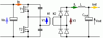
Illustration 1: Half-Bridge Push-Pull Converter

The Push-Pull converter drives the high-frequency transformer with an AC voltage, where the negative as well as the positive half swing transfers energy. The capacitor-bridge generates, in its centre point, a voltage of ½ V_in.
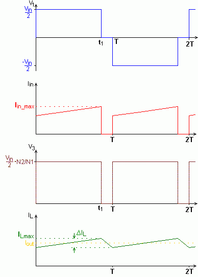
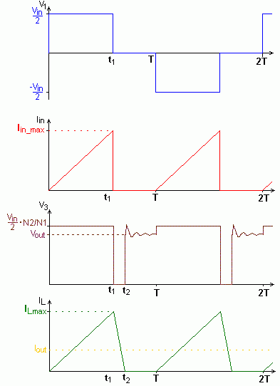
The primary transformer voltage V₁ can be +½ V_in, -½ V_in or zero depending on whether the upper transistor, the lower transistor or neither is on.
On the secondary side, the AC voltage is rectified, so that V₃ is a pulse-width-modulated voltage which switches between ½·V_in·(N₂/N₁) and zero. Due to the rectification, the pulse-frequency of V₃ is equal to 2· f .
The Low-Pass filter, formed by the inductor L and the output capacitor C_out, produces the average value of V₃. For continuous mode (I_L never becomes zero) this leads to:

The Duty cycle of this converter may theoretically increase to 100%. In practice this is not possible because the serial connected transistors, T₁ and T₂, have to be switched with a time difference to avoid a short circuit of the input supply.

Due to the fact that the duty cycle t₁/T can theoretically increase to 100%, it follows for the turns ratio that:

In the program, this value is multiplied by a factor of 0.95, so that the proposed value for N₁/N₂ includes a small margin which guarantees the demagnetisation of the core, when the input voltage is minimal, (remember: at minimum input voltage the duty cycle reaches its maximum).

Tips

• The larger the chosen value of the inductor L, the smaller the current ripple ΔI_L. However this results in a physically larger and heavier inductor.
• The higher the chosen value of the switching frequency  f , the smaller the size of the inductor. However the switching losses of the transistor also become larger as  f  increases.
• The smallest possible physical size for the inductor is achieved when ΔI_L = 2I_out at V_{in_max}. However, the switching losses at the transistors are at their highest in this state.
• Choose ΔI_L so that it is not too big. The suggestions proposed by us have adequately small current ripple along with physically small inductor size. With a larger current ripple, the voltage ripple of the output voltage V_out becomes clearly bigger while the physical size of the inductor decreases marginally.
• It is best not to alter the turns ratio N₁/N₂ proposed by us.

Mathematics used in the program

V_{in_min}, V_{in_max}, V_out, I_out and  f 

Using these parameters, the program produces a proposal for N₁/N₂ and L:

(the factor of 0.95 is taken into account to allow for the fact that the duty cycle t₁/T = 1 cannot be completely reached).






  V_F = 0.7 (Diode Forward-voltage)

  ΔI_L = 0.4I_out

From this it follows that:

1. For ΔI_L< 2I_out the converter is in continuous mode and it follows that:
   
   
   
   
   
   
   
   
   
2. For ΔI_L> 2I_out the converter is in discontinuous mode and it follows that:
   
   
   
   
   
   

Main page |	How to use the program |	Function principals |	Mathematics used in the program |	Help for HF transformer
Top of page |	Application            |	Tips              |	Literature Notes                |	Help for choking coils